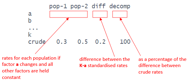
dgnpop(x = <data>,
       pop = "...",
       factors = c("..."),

       id_vars = c("..."),
       crossclassified = "...",
       ratefunction = "..."
)Standardisation and Decomposition of Rates as Products
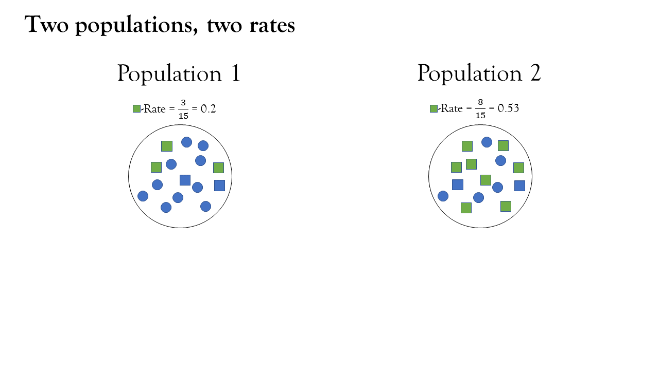
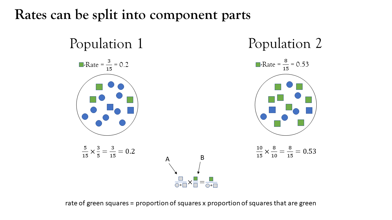
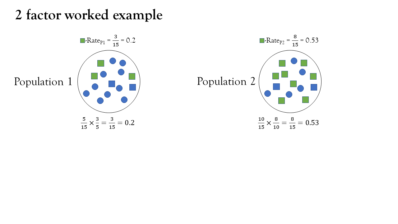
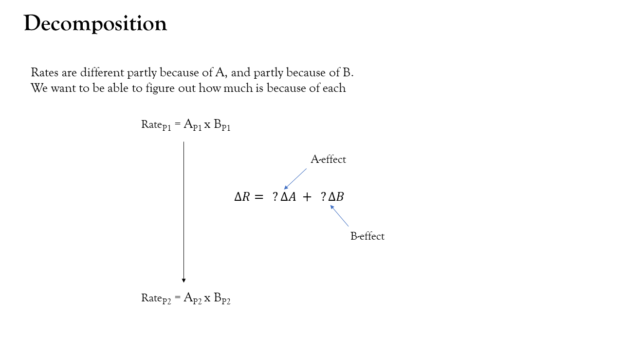
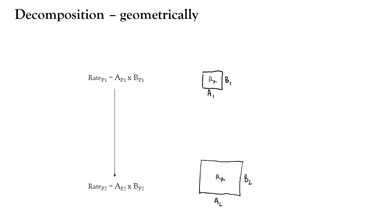
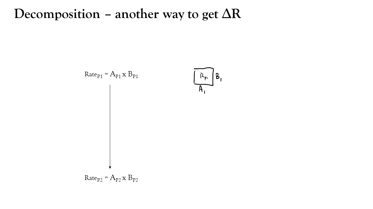
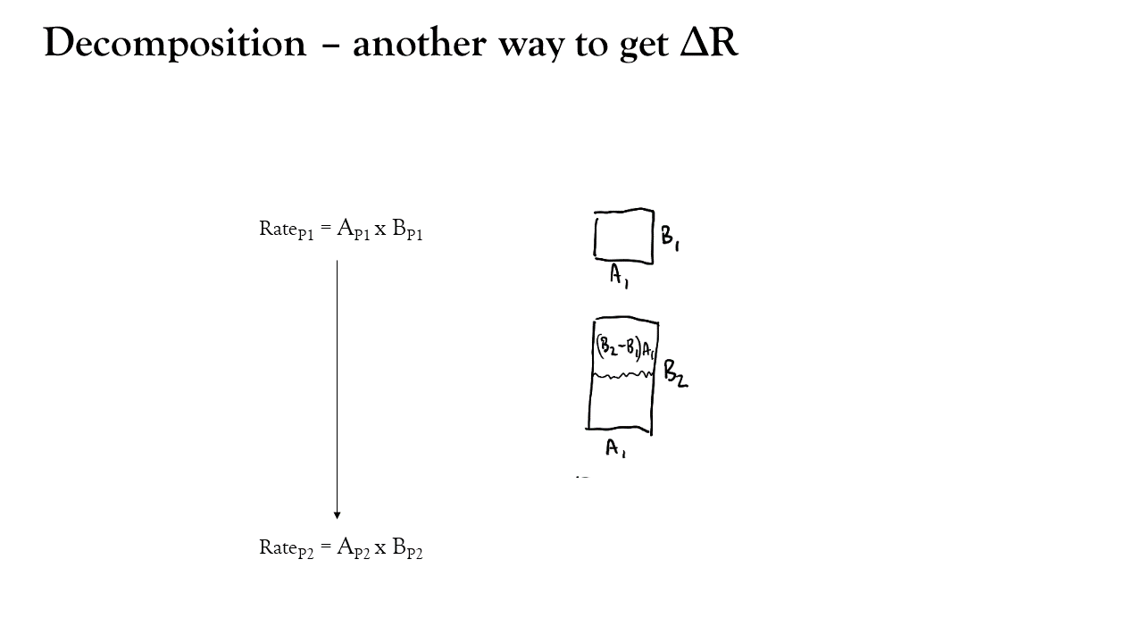
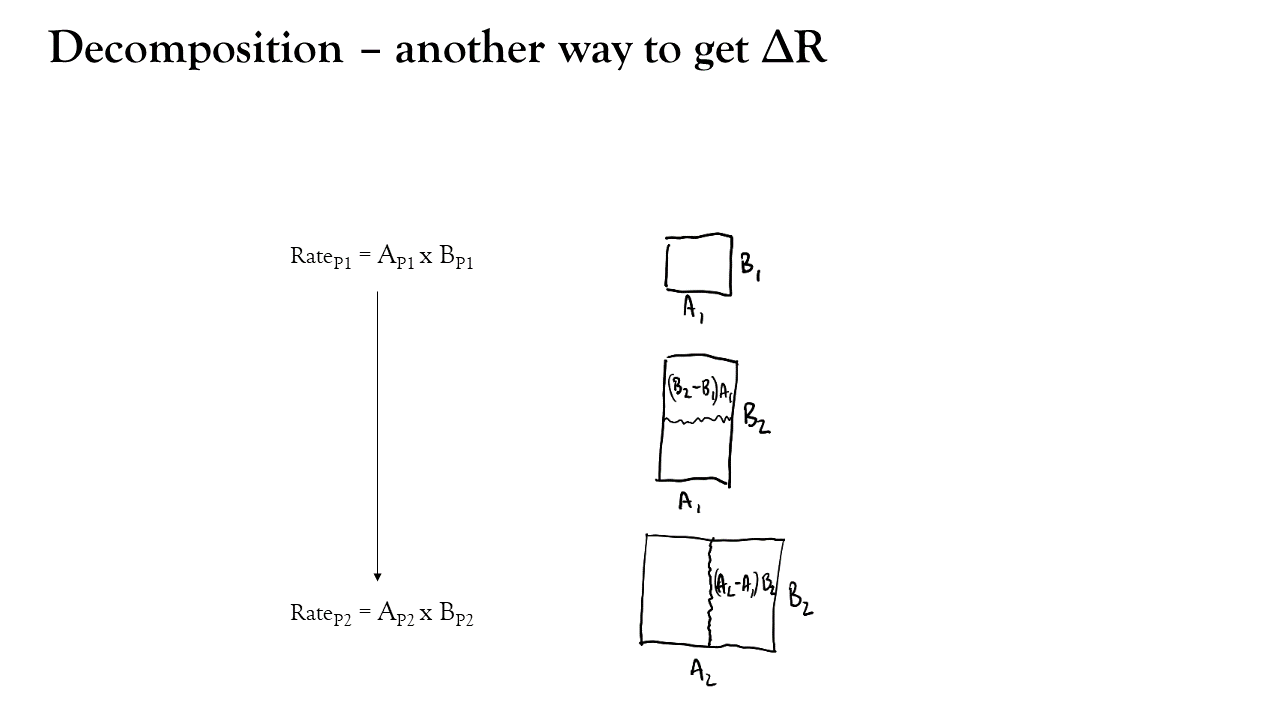
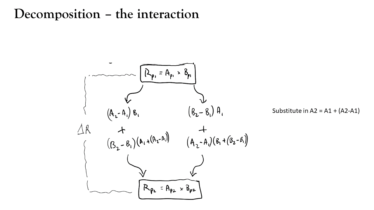
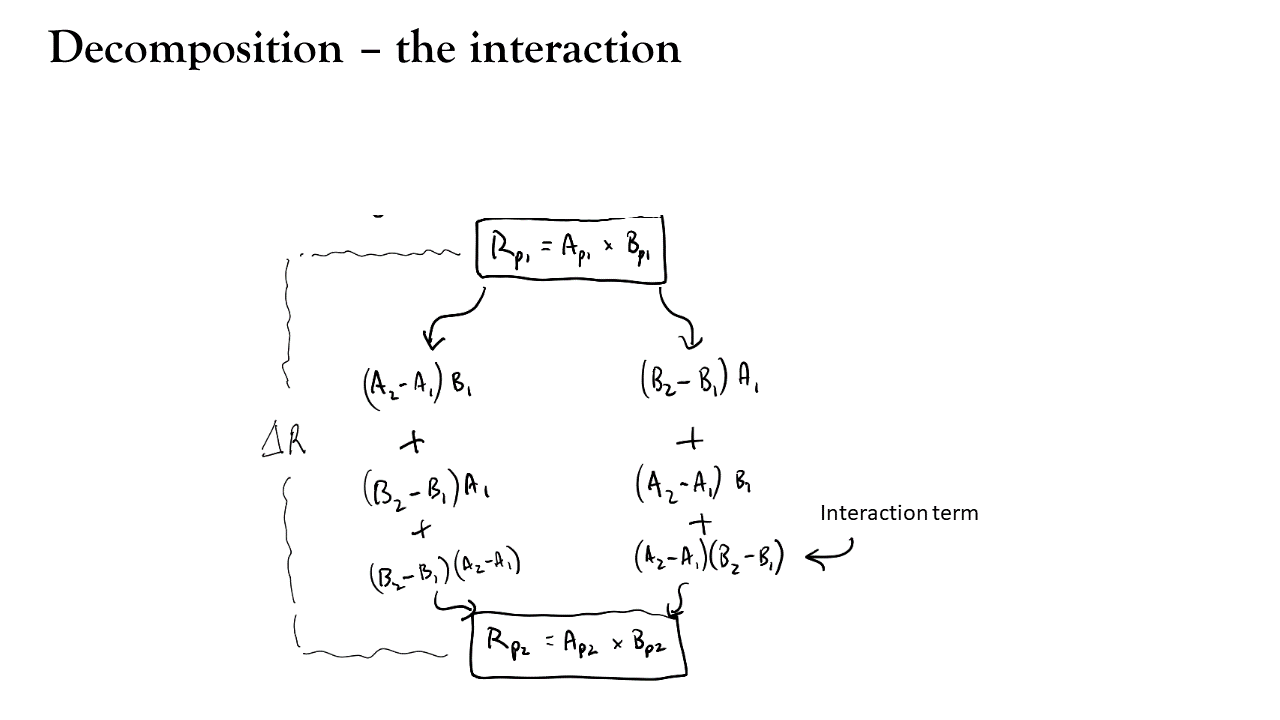
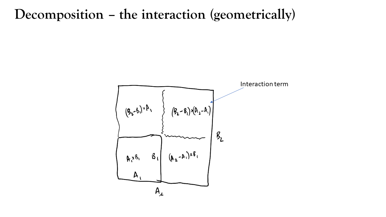
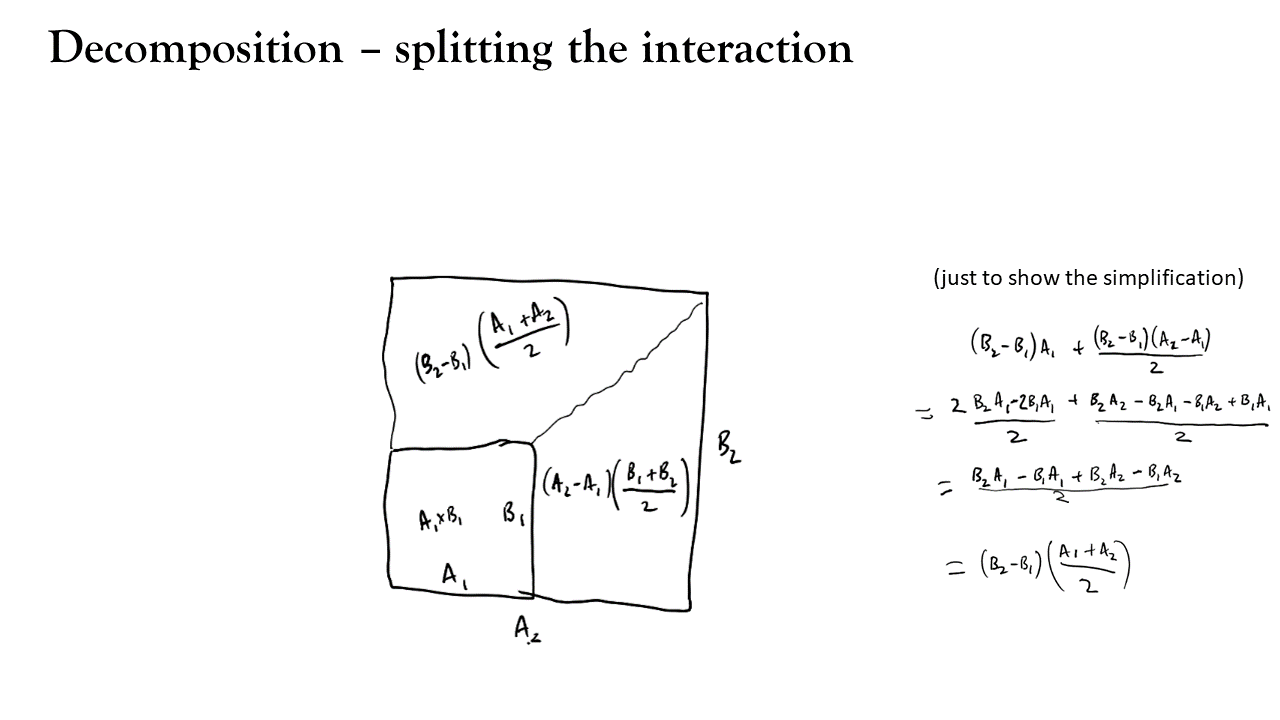
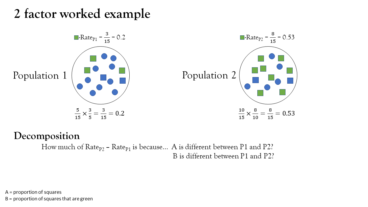
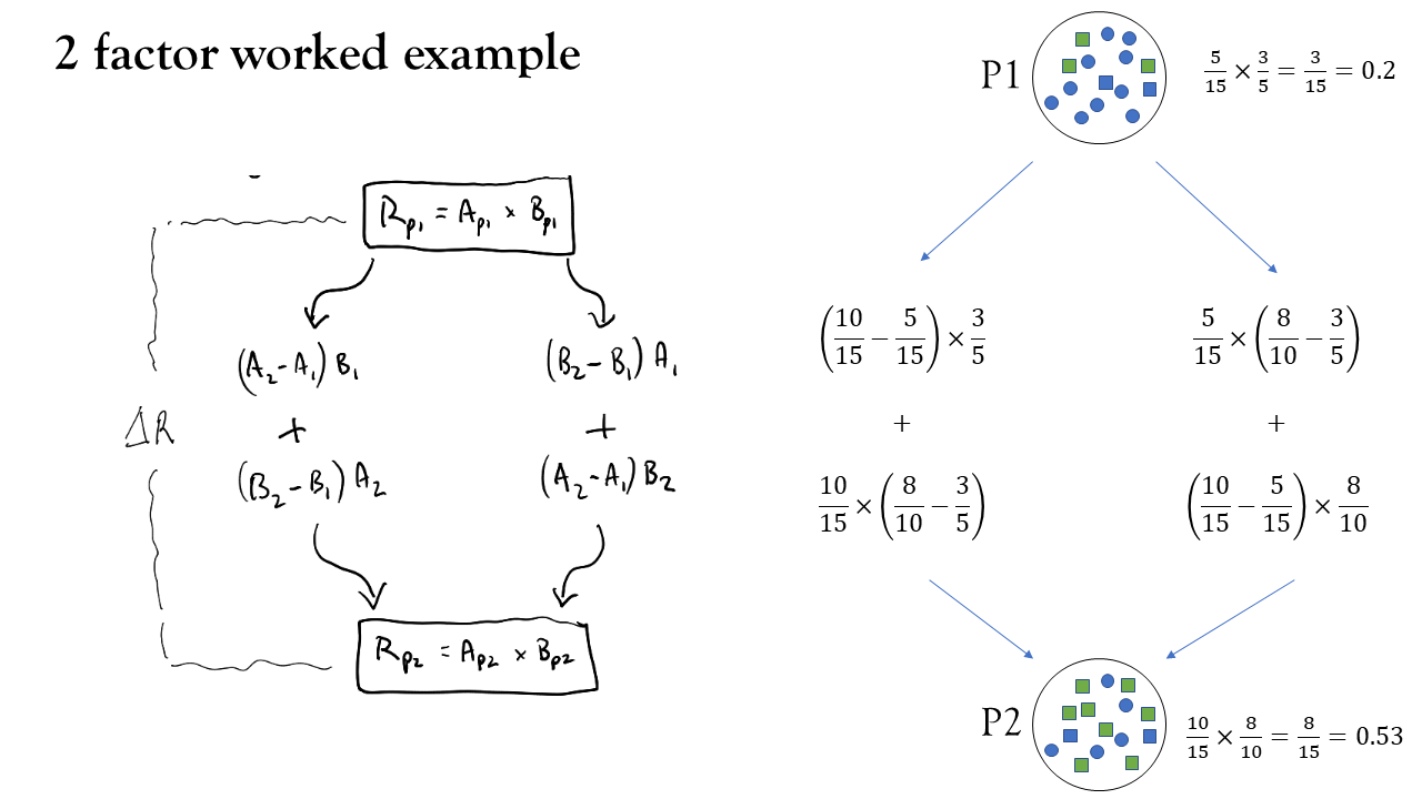
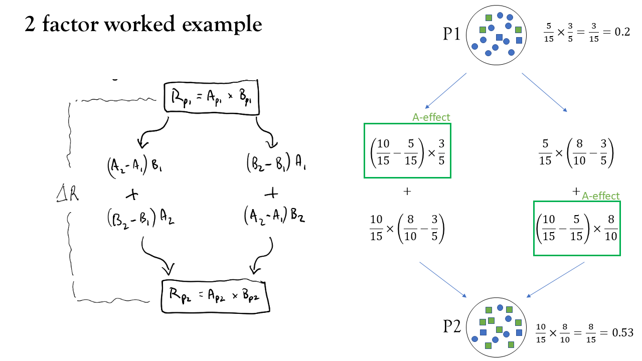
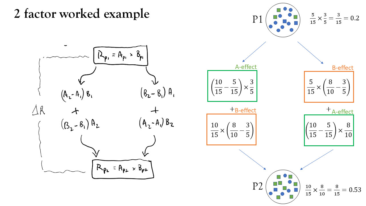
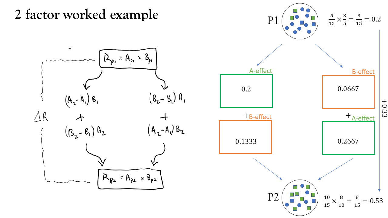
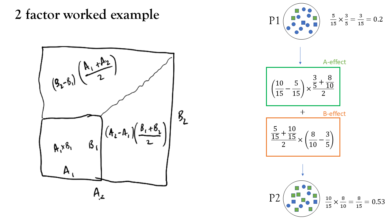
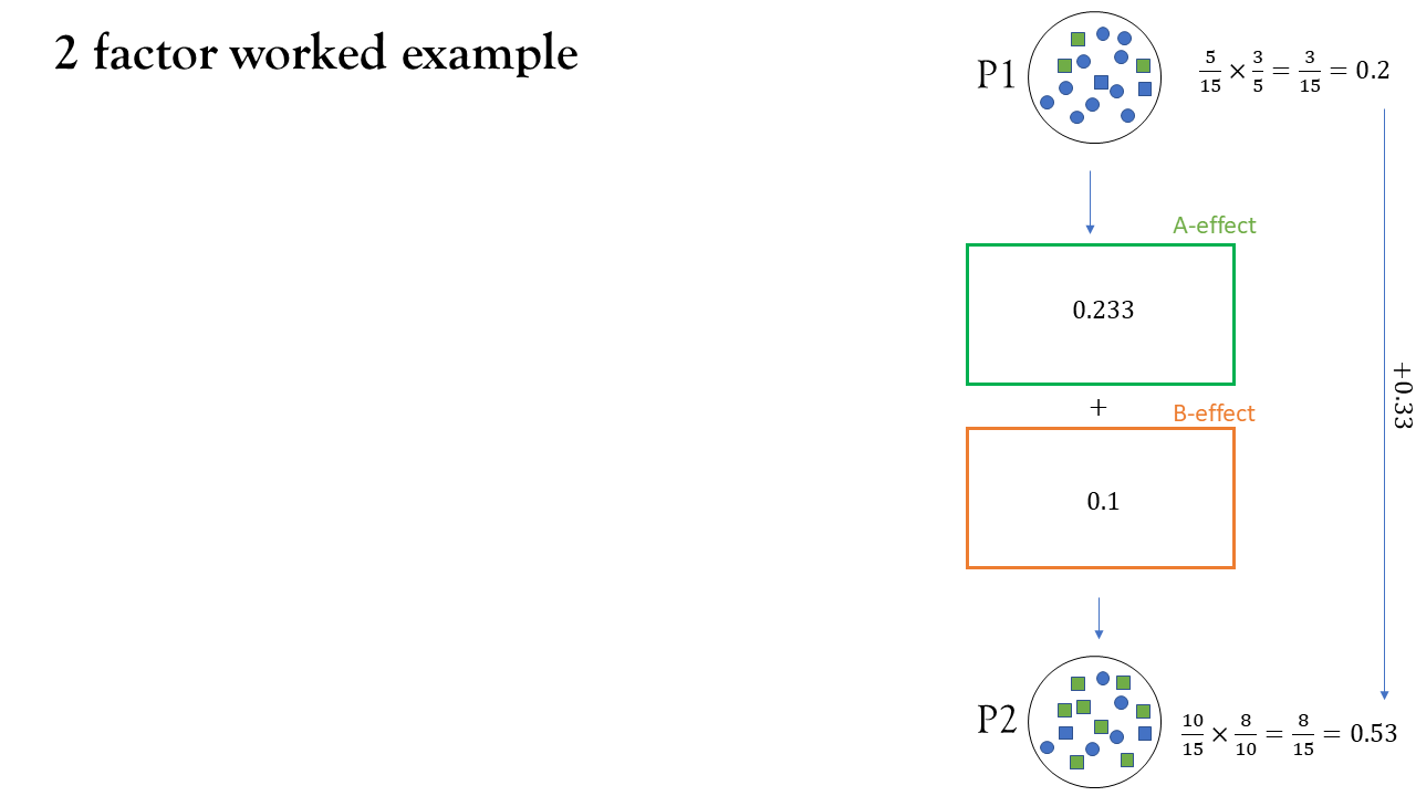
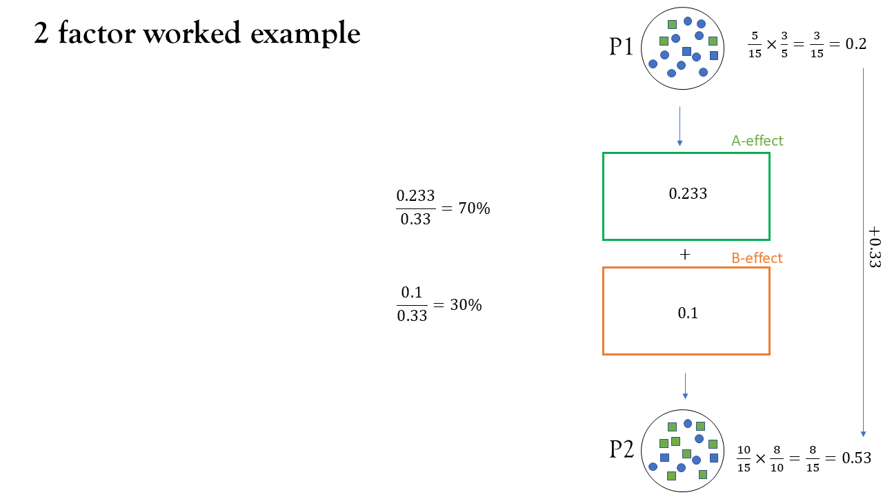
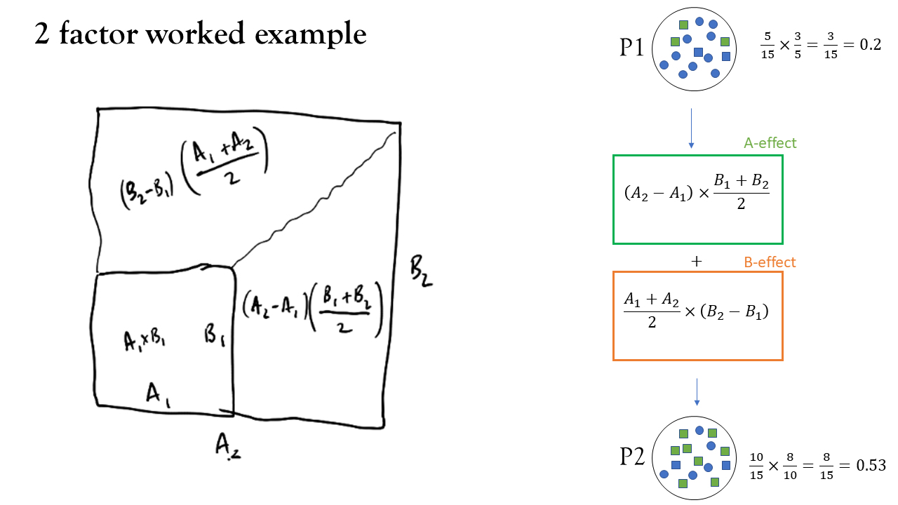
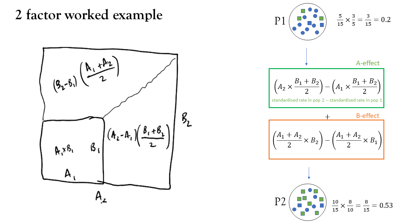
Rate as products of 2 factors\(^*\)
\(^*\) “factors” here may be better worded as “component parts”. It’s nothing to do with R’s as.factor()
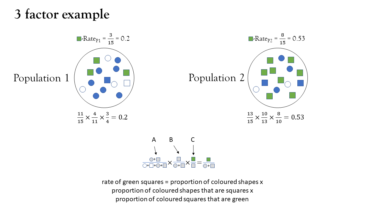
Rates as products of 3 factors
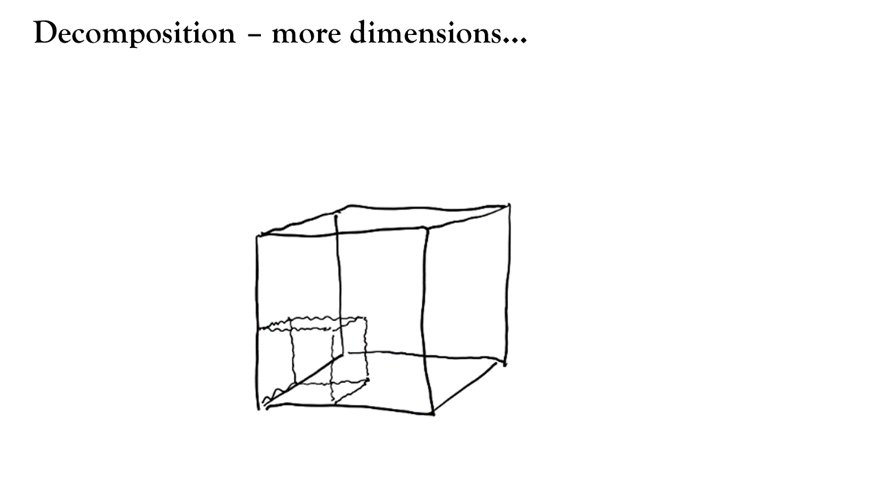
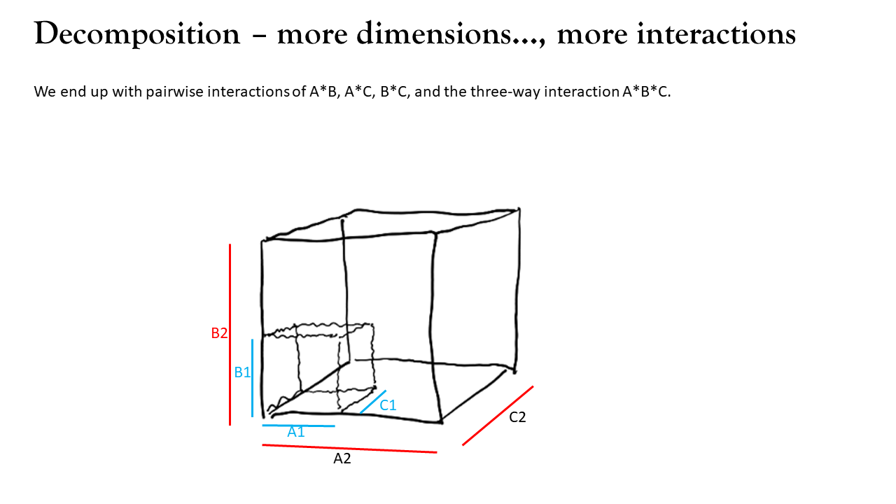
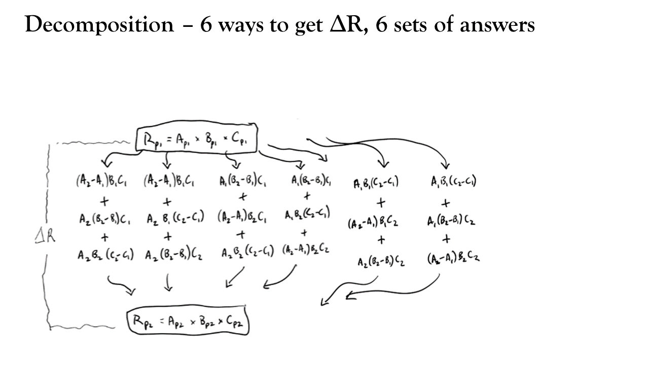
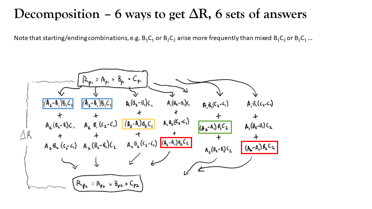
Decomposition - Das Gupta
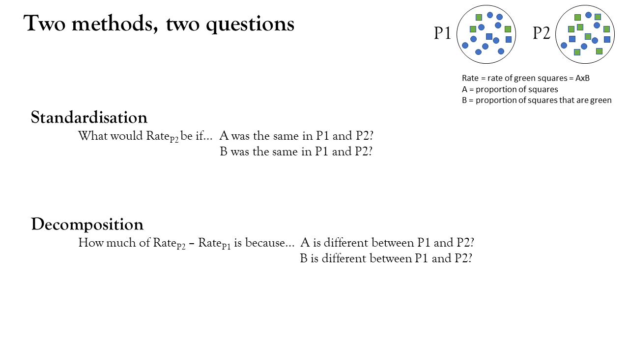
standardisation:
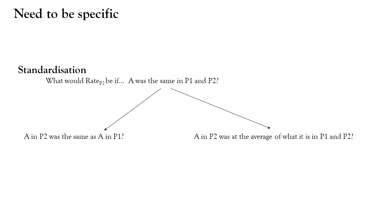
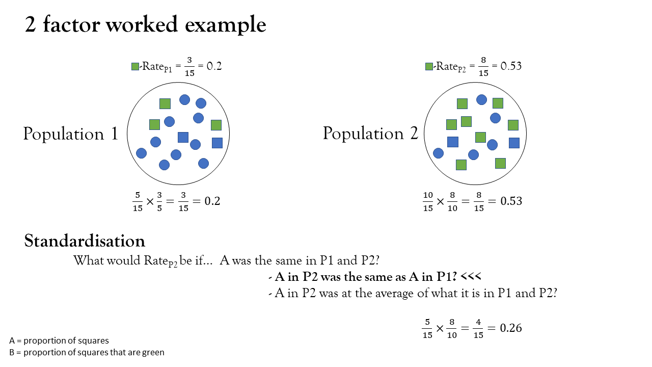
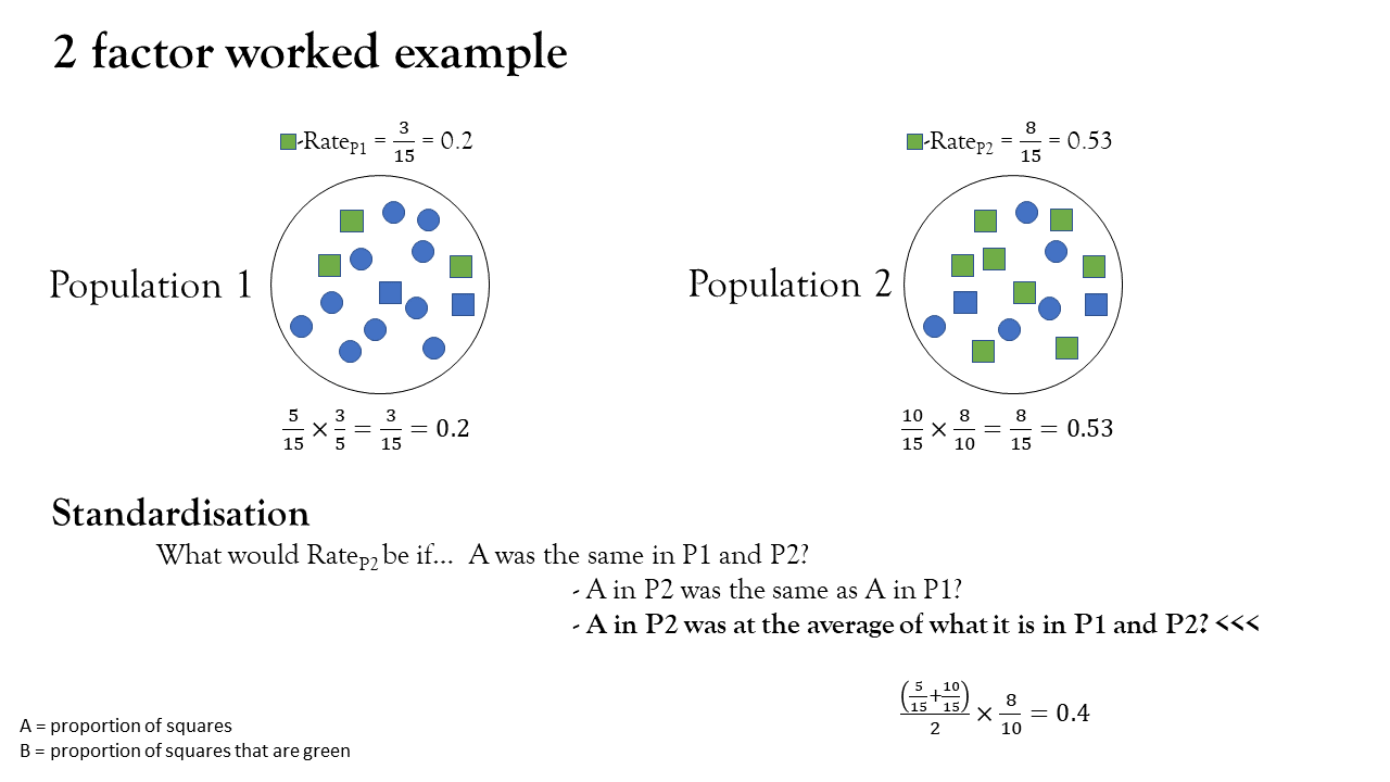
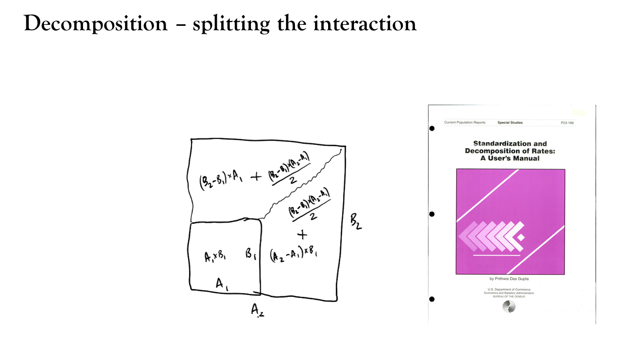
- what the rates would be if factor A was asis, but the other factors were at the average configuration’ (i.e., the weighted mean of all possible combinations of those factors across the two populations)
decomposition:
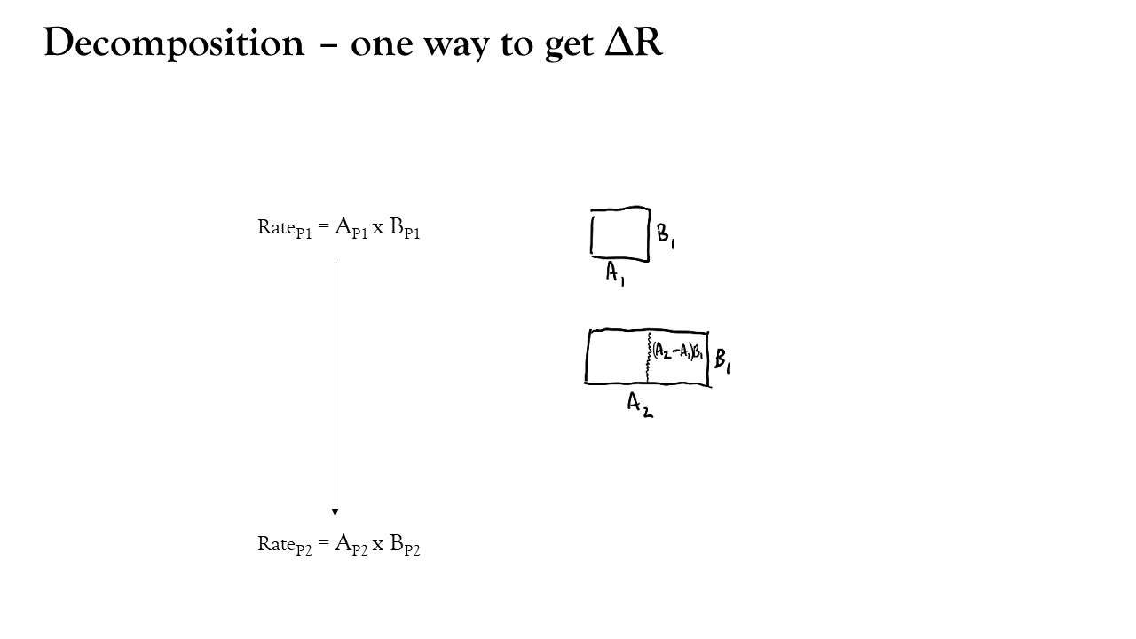
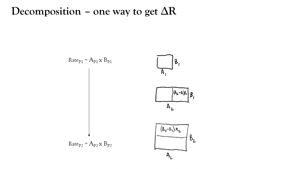
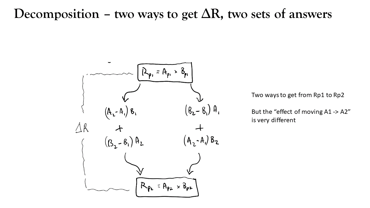
- how much of \(\Delta R\) is due to \(\Delta A\), averaged over all possible ways of moving from \(R_1\) to \(R_2\).
hypothetical rates letting one factor move and holding others constant
comparison of hypothetical rates to determine contribution of each factor
phew…

Take-away:
neutrality: doesn’t favour one population as the standard
symmetry: order of factors doesn’t matter
\(\Delta R = \Delta A_{std} + \Delta B_{std} + \ldots + \Delta K_{std}\)
Decomposition - {DasGuptR}
Why?
developed because we shared an office back in 2019.
implements all of Das Gupta’s 1993 manual:
- K factors
- arbitrary rate functions (not just products)
- crossclassified data structures
- N populations
Decomposition - {DasGuptR}
We’ve been pleasantly surprised by the usage (n.b, expectations were low!)
- Understanding tuberculosis rates in Brazil
- Comparing contribution of different factors to epilepsy burden across different sociodemographic indices
- Changes in population composition affecting rates of ‘deaths of despair’ (USA)
- Understanding the labour market. It’s in Portuguese, but this technical note from Charles Correa at the Central Bank of Brazil has some excellent examples and explanations.
Decomposition - {DasGuptR}
Workflow
Decomposition tables:
Time series plots:
Decomposition - {DasGuptR}
2 factor
  rate pop std.set factor
1 0.20  P1    <NA>  crude
2 0.53  P2    <NA>  crude
3 0.23  P1      P2    psq
4 0.47  P2      P1    psq
5 0.30  P1      P2    pgr
6 0.40  P2      P1    pgr
^ these are the rates for each population (both crude and standardised rates)
The value of the factor column denotes the part of the rate that is not held at the average.
Decomposition - {DasGuptR}
2 factor
Decomposition - {DasGuptR}
Das Gupta tables